In this series of blog posts we discuss work done to port the COVID-19 Dynamic Causal Model (DCM) to Octave, an open source tool. In other blog posts we discuss an overview of the problem, and the practical engineering side of releasing this project. The purpose of this blog post is to provide a brief overview of the theory of Dynamic Causal Modelling, especially as it pertains to COVID-19.

We structure this blog post in three separate parts. Firstly, we briefly overview what Dynamic Causal Modelling is, and what it brings to the table as a modelling technique. Following this, we give an overview of the theory of how Dynamic Causal Modelling works, especially in the context of the type of problem the COVID-19 Dynamic Causal Model (DCM) works. Finally, we walk through how the theory of Dynamic Causal Modelling is applied in the case of the COVID-19 DCM we have ported to Octave.

What do DCMs do?

Dynamic Causal Modelling is a time series modelling technique that attempts to select between (probabilistic) Dynamical Systems models to infer a model of a time series (hence the “Dynamic” part of the name).

Dynamical Systems. A Dynamical System consists of a state space, describing the state of a system at any instant, and a function that defines the evolution over time of that same state space. Dynamical systems commonly arise in physics, in modelling how celestial bodies behave, for example. In a celestial body model, each planet would have its own part of the state space describing its position, and the dynamical systems function would describe how the position of each planet is affected by each other planet’s gravity over time.

 

We call these models Dynamic Causal Models (DCMs). The advantage of Dynamic Causal Modelling over other techniques is that it infers a (probabilistic) dynamical system. This is useful for two reasons. The first is that the solution it provides is inherently causal, generative and highly explainable. The models are causal (hence the “Causal” part of the name), since a dynamical system necessarily provides a direction of causality between explanatory variables. They are generative, in the sense that once a DCM has been inferred, one can use the selected dynamical system to arbitrarily generate new data from any desired initial state. They are explainable because a dynamical system gives a full account of the relationship between explanatory variables. These are individually very valuable properties, and few techniques can claim to do all three at the same time to the same degree, least of all in the difficult domain of time series analysis. The second reason is that, because dynamic causal modelling works within a Bayesian statistical framework (as we will discuss more below), the parameters it infers for the Dynamical System are not fixed points, but probability distributions. What we mean by this is that instead of estimating one solution, Dynamic Causal Modelling (in a sense) simultaneously estimates every solution at once, and how likely each of these is in the context of our data. This is a very valuable property and gives us a much clearer picture of the limitations and bounds of our solutions.

How do DCMs work?

Dynamic Causal Modelling uses a Bayesian statistical framework to evaluate and select between competing (probabilistic) Dynamical Systems models of a time series.

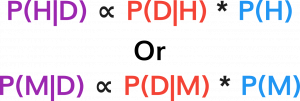
Bayesian Statistics. Bayesian Statistics is statistics based on an interpretation of probability as “reasonable expectation of propensity”. Bayesian statistics evaluates statistical hypothesis (H) (or model M) using Bayes theorem:

That is, the probability of our hypothesis (or model) given some real world data (P(H|D)) is proportional (∝) to the probability of our data given the hypothesis (or model) (P(D|H)), multiplied by our prior expectation (of the propensity) of that hypothesis (or model) being true (P(H)).

The idea is that we would like to pick between our dynamic systems models the one that is most likely to have occurred, given the data that we have. That is, for each of our dynamical systems models, we want to calculate the model M for which likelihood P(M|D) is largest using Bayes Formula.

This selection criteria is conceptually simple, but quickly runs into practical problems in the context of our Dynamical Systems models. Our Dynamical Systems models likelihood depends not just on our data D but on the parameters (or probability distributions thereof), say, θ) we choose for it. For these dynamical systems, we effectively have two problems to solve: selecting between different dynamical systems models, and for the best dynamical systems model, selecting the best choice of parameters (or distributions thereof). The second one of these is quite easy, and can be solved using analytical techniques. The first one of these however, turns out to be extremely challenging and evaluating likelihood directly is, in general, an intractable problem. For this reason, Dynamic Causal Modelling makes use of an approximation to likelihood(P(M|D)), called Free Energy.

Free Energy

There exist several well known measures (AIC or BIC for example) for approximating model likelihood, without evaluating it directly. The problem with these (non free energy) measures is that they tend to depend solely on the number of parameters in the models being compared without considering any interdependencies between parameters. Given the type of models that we are inferring in Dynamical Systems, such interdependencies are likely, and need to be accounted for. For this (and several other) reasons, Dynamic Causal Modelling uses the criterion of Free Energy as a way of evaluating an approximate likelihood score for each model. Free Energy evaluate the goodness of a model as:

Disregarding the details of the formula, we can think of free energy broken down in terms of Accuracy and Complexity. The complexity term of the equation denotes a measure of how much our current estimate of the distribution of our parameters differs from the true distribution parameters. The Accuracy term side denotes the probability of our model.

Free Energy is useful for two reasons. The first is that, as a system, it allows the accuracy and complexity of a model to be traded-off (and in a way that sensibly accounts for interdependencies between parameters). This is important, because overly complex models are generally accurate when tested, but do not generalize well. The second is that at the point at which we can find the smallest free energy (and the smallest complexity term) for a model, the free energy becomes approximately equal to the true likelihood of the model. This is particularly useful because while calculating true model likelihood directly isn’t a tractable problem, calculating this minimized free energy is.

Avoiding the details of exactly how calculating this minimized free energy (hereafter just called free energy) is achieved (variational techniques, for those interested), conceptually, we take this Free Energy and use it in place of the likelihood of our model. If we want to pick the best model, we pick the model with the highest free energy, and if we want to compare the relative likelihood of two models, we do it by comparing the ratio of their two free energies.

With Free Energy, we have a way of evaluating the goodness of a Dynamical Systems model. As we’ve said, it’s also fairly easy given such a model to calculate the best choice of parameters (or their distributions, really). The next question to ask ourselves is, given the context of the COVID-19 DCM for example, what Dynamical Systems models do we actually want to compare, and how can we do this efficiently?

Model Specification and Selection

A very common set of models we might want to compare are a given Dynamical Systems model against the same Dynamical Systems model with a certain parameter removed. We’d want to do this to see whether this parameter is useful – if the model is better without it then there is no reason to include it. For example, in our COVID-19 DCM, we might want to check a model that accounts for the effects of social distancing versus one that doesn’t, to see whether this is a useful thing to model.

It turns out that within the Dynamic Causal Modelling framework, models that are reduced versions of a model whose Free Energy has already been calculated can have their free energy calculated analytically (and quickly). This also has benefits for calculating effects across groups, as seen below.

With this in mind, a common approach in Dynamic Causal Modelling is to start with a full model that specifies all plausible parameters and connections between elements of our dynamical system, and then from this compare all reduced models to find the best scoring one. This gives us not only a sensible way to specify a space of models to score, but allows the computation of the solution to proceed efficiently.

With the system so far described, we have an excellent way of evaluating a Dynamic Causal Model for a dataset. There are many cases where we do not just have one dataset we wish to model though. In the context of the COVID-19 model, for example, we might wish to model multiple countries at once.

Group DCMs

As we’ve said, a common problem when applying Dynamic Causal Modelling in the real world is the calculation of DCMs across a population, for example modelling multiple countries in the COVID-19 pandemic. There are two easy solutions to this. In the first instance, we could simply pool all of our countries’ data together, and analyze this. The problem with this is that it discards (important) differences between countries. We could also do the opposite treat all our countries separately. The problem with this is that there are strong similarities between countries we want to benefit from using.

This is not a new problem to statistics, and one of the canonical solutions to this is to do partial pooling, in which we consider both the effects from each country on it’s own (local) and all countries together (global) simultaneously. This boils down to a hierarchical model, in which our predictions are based on both local and global effects at the same time.

Estimating both local and global effects at the same time is a difficult problem. We are fortunately able to finesse this within the Dynamic Causal Modelling framework however, with a useful observation: if we first calculate our model entirely as through it is a first level (local) model, then all the calculations we need to do calculate the full hierarchical model can be based on sub-models of this. We won’t go into the details of why this is the case, but this is exceptionally useful because, as we have observed above, evaluating sub-models of an already calculated model is very fast.

The end result of this group procedure is a DCM for each individual, say country in the case of the COVID-19 model, whose parameters are based both on the observations from that country, and the observations across all countries where appropriate.

The COVID-19 DCM

Walk through

We now move on to looking at how this theory is applied in the COVID-19 DCM specifically. Our very first step will be to define what outcomes of the pandemic it is that will be modelled. Two measures are chosen for this, number of positive tests for the virus and number of (COVID-related) deaths.

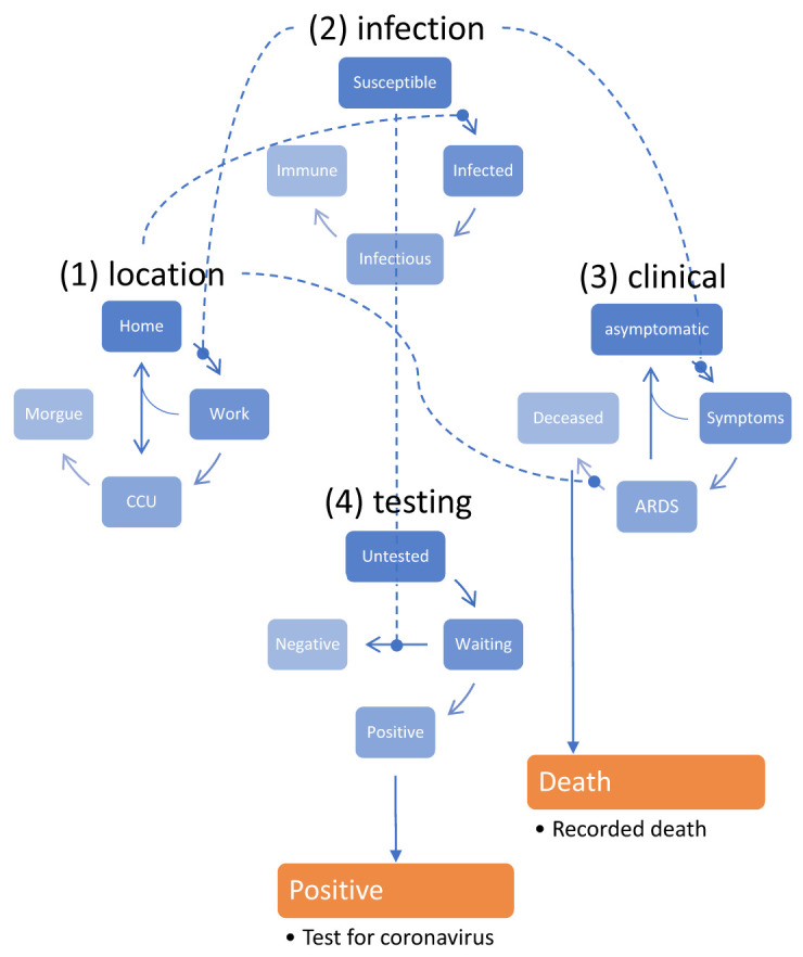
Our next step is to define what form of Dynamical Systems models we will be considering and comparing for the COVID-19 Model. In this case, this is going to be very simple – at the individual country level we are only going to consider one model. For those who might be familiar with other epidemiological models, this is essentially going to be a (complicated) SEIR model; considering each member of the population as one of Susceptible, Exposed, Infected, and Recovered. The architecture of this model can be seen in Figure 1.

In this model the state of an individual at any given time point is governed by four latent factors: Location, Infection, Clinical and Testing, each of which has four levels. Our directly measurable states in individuals are the number of positive COVID tests and the number of (COVID-related) deaths. We denote the possibility of an individual transitioning between states with the filled lines and dotted arrows, with the arrows indicating the direction of the effect. We denote an influence on a transition probability from a factor or state through a dotted line. Note that when considering these factors, the labels for each of the factors/levels are descriptive, and generally require broad interpretation. The “work” level of the location factor for example, is probably more accurately (but less snappily) considered as “not at home, the CCU or the morgue”.

As an example, consider the clinical status of the population has four levels, asymptomatic, symptomatic, ARDS and Deceased. Those who are asymptomatic have a chance of becoming symptomatic at each timestep, and the chance of this happening is based on a parameter that dictates this (as indicated by the line between the two) and the current infection status of that person. If the person is not infected, they will stay asymptomatic with probability one. If they are infected (or infection), then they will transfer to the symptomatic state based on the model parameter,θ_sym, the probability of developing symptoms.

With our Dynamical Systems defined, and no systems (yet) to select between, our next step is to calculate it’s Free Energy, and parameters (their distributions) . For the model above, performing this calculation gives us a free energy of -15701 natural units (nats). As we’ve said, we’re not (at this level) considering any competing models, so there are no alternative models to evaluate the free energy of for comparison.  However, as an example, we could consider a modification to the model above. Currently, our model includes a parameter for social distancing θ_sde, that models the effect of social distancing on various transition probabilities. Currently, the model assumes that the effect of social distancing is governed by the proportion of people infected (e.g. that people will socially distance more if more people are infected). We could justifiably argue to change this assumption to create an alternative model that has social distancing equivalently dependent on the probability of encountering an infected person. If we do this and evaluate the (minimized) free energy of this alternative model, it evaluates a of -15969 nats. Comparing the two, the original model’s free energy of -15701 is clearly substantially higher than the alternative model’s free energy of -15969 nats. This indicates that while both the original and alternative model might be theoretically justified, the evidence for the original model is better.

If we were considering our countries in isolation, without any reference to global effects, we would now be done, and could start using the DCM we have fitted to start making predictions about outcomes in the future. However, as we’ve said, we do want to consider the global context of countries. As part of this, we must then decide what aspects of our model we wish to be local effects and which we consider to be global effects. In the current version of the model, the number of initial cases and all parameters related to testing are considered to be local (country specific) effects, with all others being global effects. From this, we can calculate our DCMs with parameters accounting for both local and global data, as described in the last section.

Results

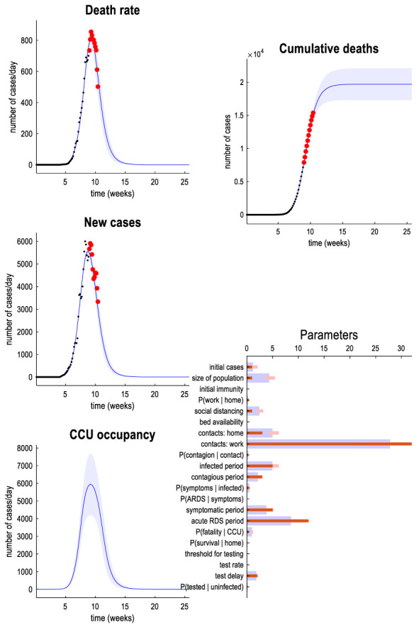
With global and local effects estimated, we have our final DCMs. To relate this back to the real world, we will burrow into one country in particular and examine predictions of the first wave of the virus based projections from the model based on early data, and how these have compared to reality in retrospect. Here we choose the UK, exploring a model of the initial outbreak based on an estimated population size of a small city (prior population estimate, 1,000,000). These can be seen visually in Figure 2.

Figure 2 shows the predictions from the model. These correspond to data taken from the first 10 weeks of the pandemic. These real world data points are given by the black dots. The blue lines denote the expected outcome according to the model. In respect of the blue shaded area, recall that what we’re actually estimating in DCMs is not an individual point estimate of parameters and outputs, but a distribution of all possible values of them and their likelihood. The blue area denotes a 90% confidence interval for the estimate of the measure. That is, that we believe there is a 90% chance that our estimate will lie within this area. The top right hand panel denotes the same as the top left hand panel, but in terms of cumulative deaths. The bottom right panel denotes estimates for the parameters of the system.

Practically, this figure gives us some predictions about how the pandemic will unfold in future. It predicts that new infections will peak about 11 weeks after the first case, with death rates and CCU occupancy peaking approximately two weeks after this. Notably, in respect of this CCU occupancy, it predicts that demand for CCU occupancy will not exceed supply. It currently predicts cumulative deaths will peak within 5 weeks, and lie with 90% confidence between 13,000 and 22,000. In terms of parameters estimated from the model, some interesting points are an estimation of the test delay (2.02 days, 90% confidence: 1.668-2.45), and the estimation of a fatality for those in the CCU (48%, 90% confidence: 39%-60%).

How does this model hold up against reality? Given that this model is aimed at the first wave of the virus but now we are substantially further along the pandemic than this initial 10 weeks of data which this model was trained on, we’re in a good position to do retrospective analysis. Comparing the model (effective population, 2.5m) against outcomes in London (population ~8.9m). Some accurate predictions:

• New cases in London will first peak on April 5th 2020
  • This was confirmed accurate, with cases first peaking on London on April 5th
• Deaths in London will first peak on April 9th 2020
  • This was also accurate, with deaths peaking at 249 on that day
• By June 12th, social distancing should no longer need to be a factor in daily life
  • Mostly accurate. Second government relaxation of lockdown was announced on June 10th (2020) and June 23rd 2020.

This said, the model has also made some incorrect predictions:

• About 12% of London’s population will have been tested by May 8th 2020. Of these, around half will be positive.
  • This was an overestimate. Actual positive tests are around ¼ of what was predicted here
• Peak daily death rate will be 807 (90% confidence 710-950) with cumulative deaths of 17,500 (90% confidence 14,000-21,000).
  • This was a substantial overestimate. Peak daily death rate was 249 (April 9th), and as of 17th July 2020, death rate was only 6106.

For a more in depth discussion on the model, with further examples see here. Overall, the model does in most respects quite a good job of modelling the outbreak, especially considering it is trained on data from across the whole country, and tested against outcomes in London specifically.

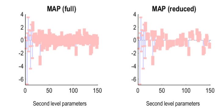
One analysis we might do further assess and improve the model is to examine which of the parameters of the model are useful. We can do this using the model selection procedure that we discussed in the previous section, but didn’t apply when we were modelling each country individually. When we apply this analysis to our full hierarchical model, we find many of our global parameters are redundant. Specifically, while the “direct” global parameters of the DCM have been retained, many of the parameters that relate global independent variables (such as latitude) to parameters that mediate transitions in the DCM model have been pruned. For example, as part of our analysis we note that the effects of a country’s latitude on the average period of Acute Respiratory Distress is a parameter that is almost entirely redundant. We can see the scope of this redundancy in Figure 3 below:

Parameters whose estimate has been reduced to zero can be considered removed. The left hand of figure 2 shows the estimates of the parameters for the full model containing all global parameters. The right hand of figure 2 shows the estimates of all the same parameters after the redundant ones have been downscaled or removed. The takeaway from this figure is that while many parameters have been retained, many have also been removed, and that many parameters that we have included in our global model are potentially redundant.

Conclusion

This work was part of a greater project by Embecosm to make the UCL model of the COVID-19 pandemic truly Free and Open Source. We discussed the overarching theory of DCMs, and worked through this theory in the example of the COVID-19 DCM, modelling the COVID-19 pandemic. Those interested in the practice may find either the practical blogpost or the repository interesting.